Weight initialization - impact on layer distribution

2017, Jul 25

In this post, I will carry out some experiments to demonstrate the impact of weight initialization on the distribution of activations on each layer in neural network, especially the very last layers. This was mentioned by Andrej in cs231n/lec6 as a motivation paving the way for batch normalization.

I will try to keep things simple with intuition. Mathematics will not be richly convered.

1. Covariate shift

1.1. What is Covariate shift?

Covariate shift refers to changes in the distribution of input variables. This shift is usually addressed as a problem causing poor performance in training neural networks.

Note: In the context of neural networks, a layer takes the activations of the previous layer as its input. Therefore, it is also equivalent if we investigate the distribution of activations of a layer.

1.2 .What does it look like?

Consider a neural networks with 20 fully connected layers.

Input shape: 49000x3072 (reshape from 49000 CIFAR images of size 32x32) and was whitened (zero-centered & normalized).
Hidden layers: 19 layers of shape (100, 100)
Activation function: ReLU.
Biases: all zeros.
Weights: normal distribution, scaled by factor 0.1.

The distributions of layer ouputs are illustrated in the figure below. We can apparently see that the variance constantly decreases in deeper layers.

Fig 1. Distribution of activations in layer 1, 3, 5, 7.

1.3. Impact of Covariate shift?

When training a network, if the activations fall in a narrow range like above, the gradient on those activations could be relatively small, leading to gradient saturation/vanish. Training gets stuck as a result. We sometimes face the same problem with dispersing distribution.

2. Param initialization

Param initialization is a primary cause of covariate shift. We will focus on weight initialization, and let biases be all zeros.

An initialization strategy is considered good if it maintains the same mean and variance (or standard deviation) throughout layers. Since the input data was whitened, we expect mean around zero (+/-1), std around 1 (+/-0.5).

$\mu = 0.3, \sigma = 0.7$ ⟶ accepted ✅
$\mu = 0.3, \sigma = 0.003$ ⟶ NOT accepted ❌
$\mu = 15, \sigma = 320$ ⟶ NOT accepted ❌

2.1. Setup

Some setup code for experiments:

def relu(x):
    return np.maximum(x, 0)

def forward(X_flat, hid_dims, weights, biases, activation=relu):
    """
    Feed forward.
     - X_flat: shape: N x D, where D = d1 x ... x dk.
     - hid_dims: 1D array.
     - weights: array of weights: W1, W2, ...
     - biases: array of biases: b1, b2, ...
     - activation: activation on each layer. None if no activation.
    """
    assert len(weights) == len(biases), 'weights and biases must have the same length'
    assert len(hid_dims) + 1 == len(weights), 'len(weights) must equal len(hid_dims) + 1'

    all_layers = []
    out = X_flat
    for l in range(len(hid_dims) + 1):
        out = np.dot(out, weights[l]) + biases[l]
        if activation is not None:
            out = activation(out)
        all_layers.append(out)

    return out, all_layers

def visualize_distribution(all_activations):
    n_layers = len(all_activations)
    activations_mean = [np.asscalar(np.mean(activations)) for activations in all_activations]
    activations_std = [np.asscalar(np.std(activations)) for activations in all_activations]

    xs = range(1, n_layers+1)
    _, axes = plt.subplots(2, 2, figsize=(8, 8))
    ax1, ax2, ax3, ax4 = axes[0, 0], axes[0, 1], axes[1, 0], axes[1, 1]
    ax1.plot(xs, activations_mean, '-o', color='#0067a7')
    ax1.set_title('means by layer')
    ax1.set_xlabel('layer')
    ax2.plot(xs, activations_std, '-o', color='red')
    ax2.set_title('std by layer')
    ax2.set_xlabel('layer')

    ax3.hist(all_activations[14].ravel(), bins=50, color='green')
    ax3.set_title('Distribution of layer 15')
    ax4.hist(all_activations[-1].ravel(), bins=50, color='green')
    ax4.set_title('Distribution of the layer %d' % n_layers)

    plt.tight_layout()
    plt.show()

    # Print mean and std of last 5 layer
    for l in range(n_layers)[-5:]:
        print('Layer %2d. mean: %f\tstd: %f' % (l+1, activations_mean[l], activations_std[l]))

def initialize_params(in_dim, hid_dims, out_dim,
                      weight_initializer=np.random.randn,
                      bias_initializer=np.zeros):
    dims = [in_dim] + hid_dims + [out_dim]
    weights, biases = [], []
    for l in range(len(hid_dims) + 1):
        w = weight_initializer(dims[l], dims[l+1])
        b = bias_initializer(dims[l+1])
        weights.append(w)
        biases.append(b)
    return weights, biases

def examine_distribution(weight_initializer, activation=relu, n_layers=20):
    in_dim, out_dim = 32*32*3, 10
    hid_dims = [100 for i in range(n_layers - 1)]

    weights, biases = initialize_params(in_dim, hid_dims, out_dim,
        weight_initializer=weight_initializer)

    _, all_activations = forward(X_train_normalized, hid_dims=hid_dims, 
        weights=weights, biases=biases, activation=activation)

    visualize_distribution(all_activations)

Now, lets examine some initialization schemes…

2.2. Trival initialization

The common way is using normal randomization with a scale. This scale should equal the standard deviation of the random numbers.

def trivial_initializer(d1, d2, weight_scale=0.1):
    return np.random.normal(0, weight_scale, (d1, d2))

examine_distribution(trivial_initializer)

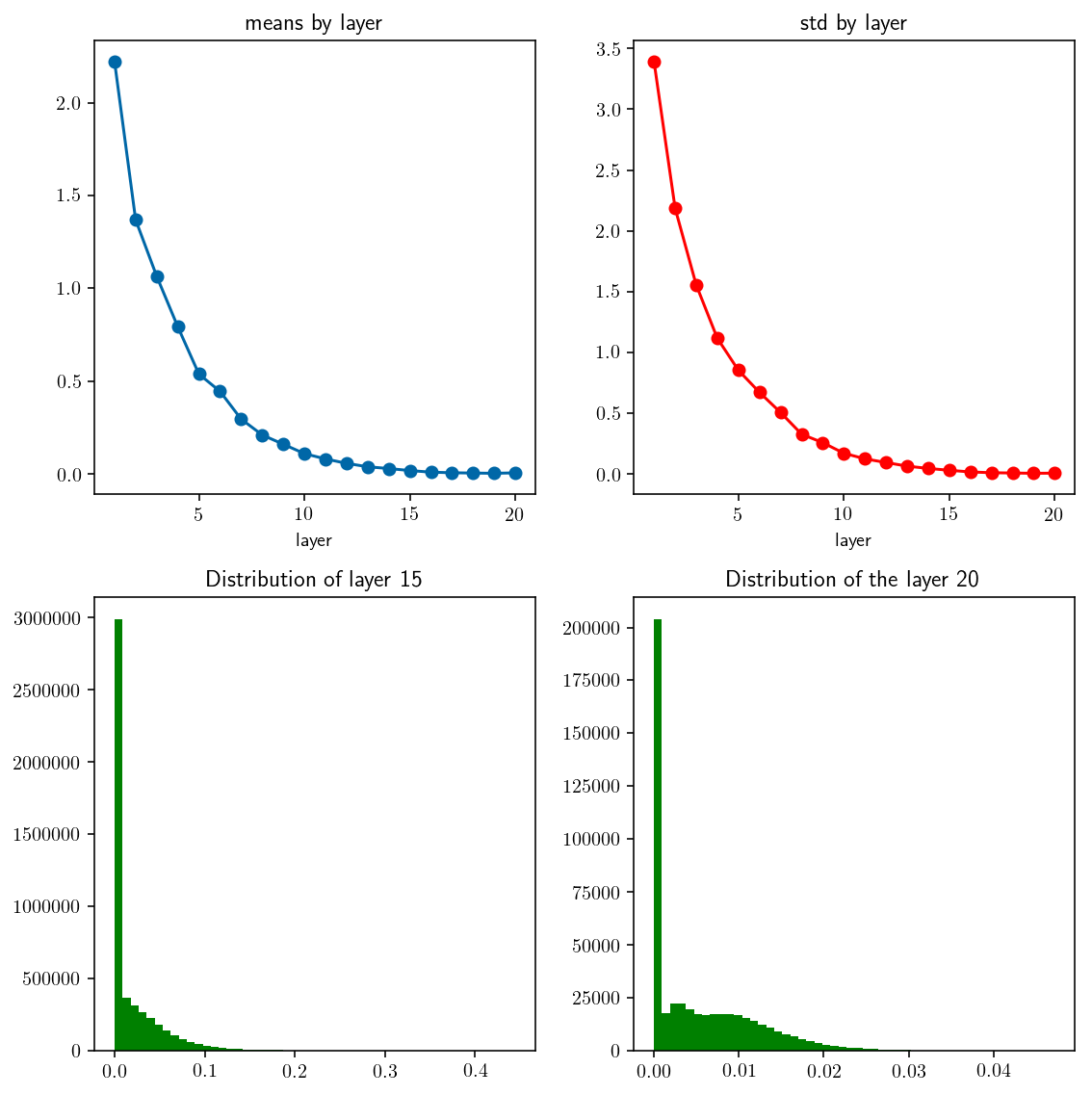
Fig 2. mean and std by layer. Initialized by Gaussian $\mu=0, \sigma^2=0.1$.

Layer 16. mean: 0.009006    std: 0.016165
Layer 17. mean: 0.005849    std: 0.009699
Layer 18. mean: 0.004207    std: 0.007308
Layer 19. mean: 0.002917    std: 0.004961
Layer 20. mean: 0.005232    std: 0.006176

⟶ Not accepted ❌

examine_distribution(lambda d1, d2: trivial_initializer(d1, d2, weight_scale=0.2))

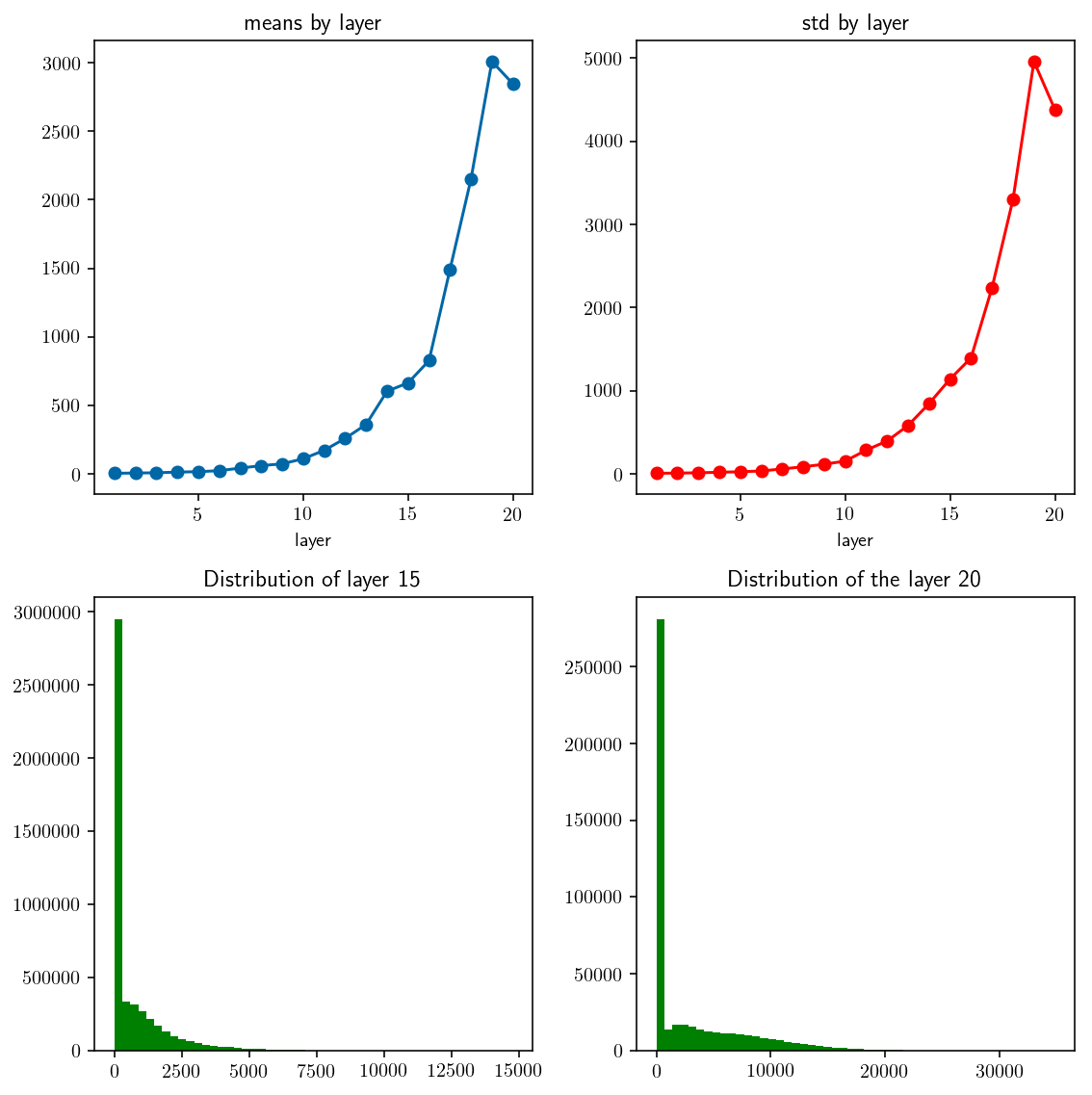
Fig 3. mean and std by layer. Initialized by Gaussian $\mu=0, \sigma^2=0.2$.

Layer 16. mean: 825.965548	std: 1394.566496
Layer 17. mean: 1491.038728	std: 2237.786857
Layer 18. mean: 2149.680649	std: 3300.200497
Layer 19. mean: 3008.496905	std: 4961.155125
Layer 20. mean: 2845.114905	std: 4381.190124

⟶ Not accepted ❌

Notice that after changing weight scale from 0.1 to 0.2, how output values are distributed changed radically. Quite sensitive to weight scale, huh?

2.3. Xavier initialization (Glorot initialization)

This scheme is based on the observation that:

$$\begin{equation} var(s) = var(\sum_i^N{w_i.x_i}) = … = N.var(w).var(x) \end{equation}$$

In order to keep the same variance, we need: $var(w) = 1/N$. So, the weight scale should be $\sqrt{1/N}$

def xavier_initializer_1(d1, d2):
    return np.random.randn(d1, d2) * np.sqrt(1.0 / d1)

examine_distribution(xavier_initializer_1, activation=None)

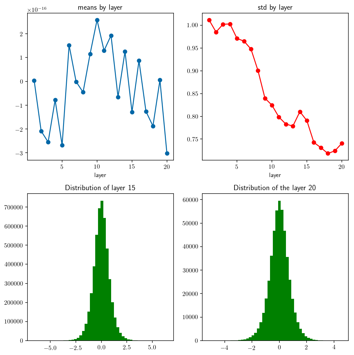
Fig 4. mean and std by layer. Initialized using xavier initialization, with no activation.

Layer 16. mean: 0.000000	std: 0.742681
Layer 17. mean: -0.000000	std: 0.731260
Layer 18. mean: -0.000000	std: 0.718502
Layer 19. mean: 0.000000	std: 0.724088
Layer 20. mean: -0.000000	std: 0.740663

⟶ Accepted ✅

We can see that xavier initialization gives a really nice distribution: gaussian shape, reasonable mean and std. However, this initialization strategy seems not to work well with non-linear activation. If we use ReLU as the activation function, we got a poor distribution.

examine_distribution(xavier_initializer_1, activation=relu)

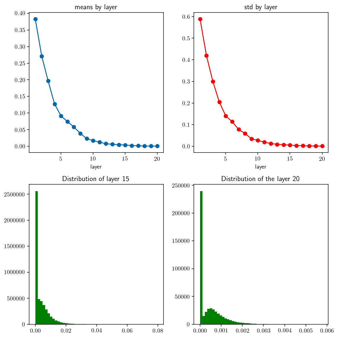
Fig 5. mean and std by layer. With relu activation, normal distribution, $var(w) = 1/N$.

Layer 16. mean: 0.002048	std: 0.003093
Layer 17. mean: 0.001338	std: 0.002246
Layer 18. mean: 0.000834	std: 0.001481
Layer 19. mean: 0.000434	std: 0.000776
Layer 20. mean: 0.000440	std: 0.000590

⟶ Not accepted ❌

A recent paper by He et al dove into the analysis with ReLU activation and finally reached the conclusion that the variance of weights should be $2/N$. This is often used in practice.

def xavier_initializer_2(d1, d2):
    return np.random.randn(d1, d2) * np.sqrt(2.0 / d1)

examine_distribution(xavier_initializer_2)

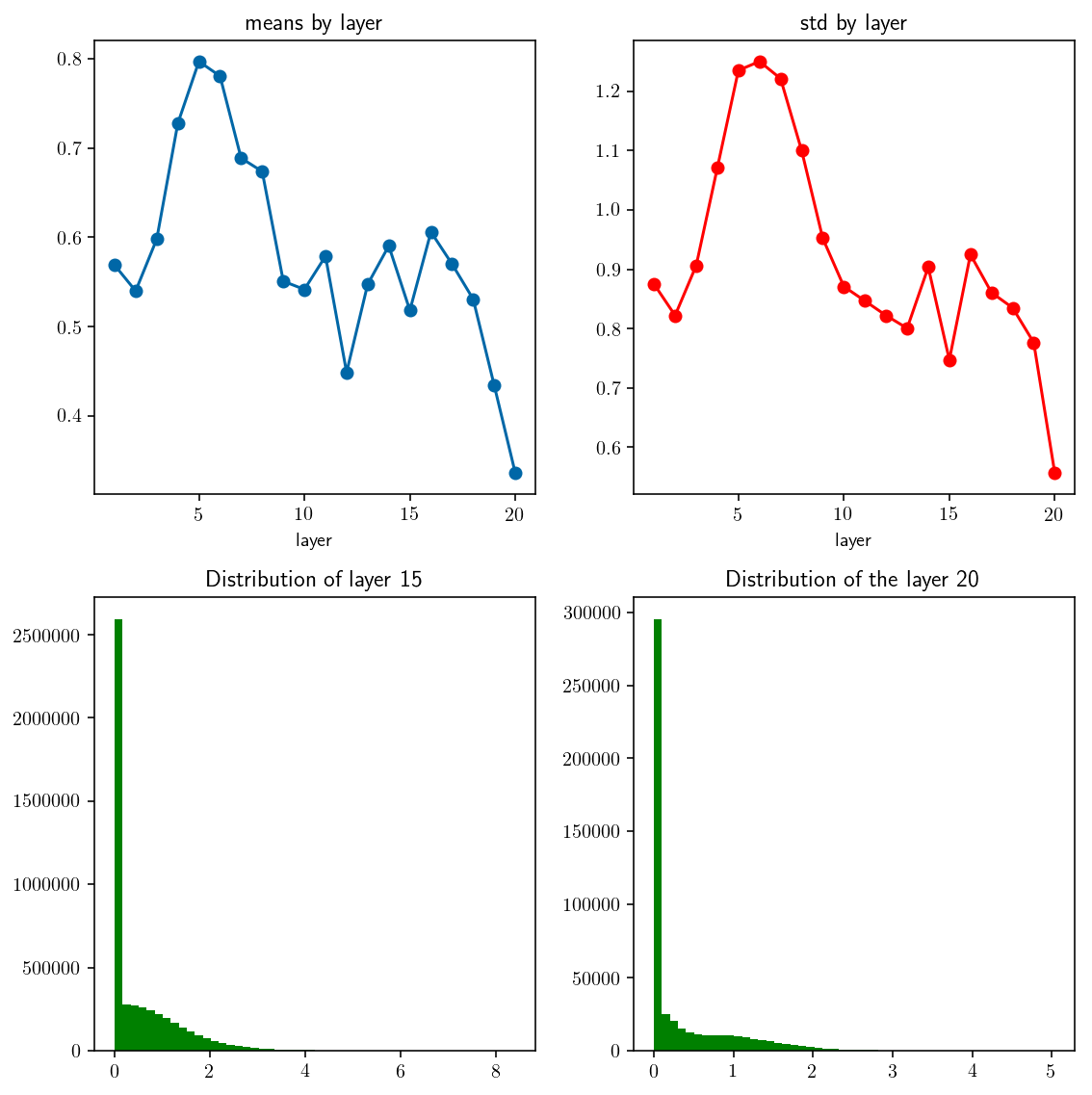
Fig 6. mean and std by layer. With relu activation, normal distribution, $var(w) = 2/N$.

Layer 16. mean: 0.605864	std: 0.924794
Layer 17. mean: 0.569898	std: 0.860651
Layer 18. mean: 0.530719	std: 0.835036
Layer 19. mean: 0.433965	std: 0.776518
Layer 20. mean: 0.335705	std: 0.556218

⟶ Accepted ✅

3. Another approaches

Another technique was recently developed called batch normalization. We will take a look at it later. P/s: A huge advantage of batch normalization is that it is more robust to bad initialization. In fact, using different values of weight scale does not produce much significant performance (and it’s already good). Therefore, tuning hyperparams would be less painful.

4. Conclusion

We have discussed covariate shift and its impact on training performance. With a proper scheme of initialization, the training could be less likely to get into this problem. We also have a look at some examples to see the distribution of activations corresponds to different schemes of initialization.

Hope this post provides helpful visualization to help understand some problems of neural networks.

Reference:

Source code: here

tech

neural-networks